LDA integrals in the clustering of SNPs and the genotypes of m0 and m2 in P1 and P2
LDA therefore takes an expected value of 0 when haplotypes are randomly assigned at different SNPs and positive values when the ancestries of the haplotypes are correlated.
Stage 2: We then explored different combinations of positive, balancing and negative selection of m0 in P1 and P2. m0 reached 80%, 50%, and 20% when it was positively selected, and then underwent balancing selection, or was negatively selected, for the next 2, 900 samples that were used as reference samples.
We investigated balancing selection at two loci as well. The balancing selection in P1 and P2 ensured that the mutant allele reached around 50% frequency, while positive selection made the mutant allele become almost the only allele. In P3, if m1 or m2 was positively selected, its frequency reached greater than 80% regardless of whether the allele experienced balancing or positive selection in P1 or P2, because we set strong positive selection. If the balancing selection for m1 was done in P1, it had a frequency of 25%, but it reached 37.5% after 20 generations in P3.
The integral ({\int }_{{\rm{gd}}\left(\,j\right)-X}^{{\rm{gd}}\left(\,j\right)+X}{\rm{LDA}}\left(\,j,l\right)d{\rm{gd}}) is computed assuming linear interpolation of the LDA score between adjacent SNPs.
LDAS(, jrm);X is a way of using left- and right-hand keys. int _gd(,j)-XrmtgrmLDA
The average distance between ancestry at SNPs explained more variance than expected in htx model selection for the ith genome
The origin of risk to be identified with multiple ancestry groups, which does not need to be a single set for each SNP, could be accounted for by a new statistics developed to understand risk-conferring haplotypes.
A strong signal of selection is the historical trajectory of SNP frequencies. The main goal of our pathway painting method is to infer selection at individual genes and combined with a polygenic score by analyzing sets of SNPs associated with a trait.
The average L2 norm is defined as the distance between ancestries at those SNPs. Specifically, we compute the L2 norm for the ith genome as
We visualized the out-of-sample R2 for each of the best models selected using the procedure described in the htx model selection procedure for smaller haplotypes. In both ‘lm’ and ‘glm’, HTRX had equal predictive performance to the true model. It performed as well as GWAS when interaction effects were absent, explained more variance when an interaction was present and was significantly more explanatory than HTR. When rare SNPs are included, interaction is rare. The difference between the two was larger as expected, and removing the rare haplotypes reduced the performance.
Notably, two SNPs stood out for explaining much more variance than the others when fitting the GWAS model using the genotype data, but overall more SNPs from GWAS painting explained more than 0.1% of the variance, which indicates that the painting data are probably more efficient for estimating the effect sizes of SNPs and detecting significant SNPs. The SNPs that use painting data explained the same amount of variance, suggesting that they are very similar.
A two-parameter approach to the largest variance in population models with age and principal components: an overfitting approach with its own pseudo-R2 value
$${O}{i}=\mathop{\sum }\limits{c=1}^{20}{\beta }{c}{C}{{ic}}+\gamma \left(\mathop{\sum }\limits_{j=1}^{4}{\beta }{{G}{j}}{G}{{ij}}+{\beta }{{H}{1}}{H}{1}\right)+{e}_{i}+w,$$
Start a model that has 18 principal components, sex and age, and perform forward regression on the subset, before adding a feature to explain the largest variance.
L0 is the likelihood of the null model. We use the adjusted McFadden’s pseudo-R2 value by taking overfitting into account.
There’s a left and a right in this picture.
$${Y}{i} \sim {\rm{Binomial}}\left(1,{\pi }{i}\right){\rm{;}}\log \left(\frac{{\pi }{i}}{1-{\pi }{i}}\right)={\beta }{j}{X}{ij}+\mathop{\sum }\limits_{c=1}^{{N}{c}}{\gamma }{c}{C}_{ic},$$
$${H}_{ij}=\left{\begin{array}{ll}1, & {\rm{if}}\,i{\rm{th}}\,{\rm{individual}}\,{\rm{has}}\,{\rm{haplotype}}\,j\,{\rm{in}}\,{\rm{both}}\,{\rm{genomes}},\ \frac{1}{2}, & {\rm{if}}\,i{\rm{th}}\,{\rm{individual}}\,{\rm{has}}\,{\rm{haplotype}}\,j\,{\rm{in}}\,{\rm{one}}\,{\rm{of}}\,{\rm{the}}\,{\rm{two}}\,{\rm{genomes}},\ 0, & {\rm{otherwise}}.\end{array}\right.$$
Step 1 is to select candidate models. The model search problem can be solved by getting a set of models that are more diverse than what was obtained using bootstrap resampling83.
The data should be randomly sampleed a subset. When the outcome is non-determining, the subset has the same number of cases and controls as the whole dataset.
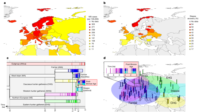
Source: Elevated genetic risk for multiple sclerosis emerged in steppe pastoralist populations
Predictors of gene-coding in steppe pastoralist populations: Experiments with a data set of SNPs, ancestries and haplotypes
In the ten folds, use different groups as the test and training dataset. The candidate models are fitted to the training dataset and then used to compute the additional variability explained by features in the test dataset. Finally, select the candidate model with the highest average out-of-sample R2 as the best model.
For MS, we used data from ref. 4. For non-MHC SNPs, we used the ‘discovery’ SNPs with P(joined) and OR(joined) generated in the replication phase. We searched the literature for reports of MHC alleles and amino acid polymorphisms. In total, we generated 205 SNPs that were either fine-mapped or in high LD with a fine-mapped SNP (15 MHC, 190 non-MHC).
The population structure in the UK Biobank 81 was captured by using 20 predictors in GWAS models, including sex, age and the first 18 principal components.
The total variance of a trait explained by genotypes (SNP values), ancestry and haplotypes (described below) is a measure of how well each captures the causal factors driving that trait. We therefore computed the variance explained for each data type in a ‘head-to-head’ comparison at either specific SNPs or SNP sets. We describe the model and covariates in this section.
We then ran a transformation step as in ref. 79, centring results around the ancestral mean (that is, all ancestries) and reporting as a Z score. To obtain 95% confidence intervals, we ran an accelerated bootstrap over loci, which accounts for the skew of data to better estimate confidence intervals80.
Source: Elevated genetic risk for multiple sclerosis emerged in steppe pastoralist populations
WAP for the kth ancestry of the SNP and the prevalence of MS in the mth cluster of SNPs
$${f}{\left{{\rm{anc}},i\right}}=\frac{{\sum }{j}^{{M}{{\rm{effect}}}}{\rm{painting}}{{\rm{certainty}}}{\left{j,i,{\rm{anc}}\right}}}{{\sum }{j}^{{M}{{\rm{alt}}}}{\rm{painting}}{{\rm{certainty}}}{\left{j,i,{\rm{anc}}\right}}+{\sum }{j}^{{M}{{\rm{effect}}}}{\rm{painting}}{{\rm{certainty}}}{\left{j,i,{\rm{anc}}\right}}},$$
We can then compute the WAP, which summarizes these results into the ancestries. For the jth SNP, let ({P}{{jkm}}={n}{{jm}}{\bar{P}}_{{jkm}}) denote the sum of the kth ancestry probabilities of all the individuals in the mth cluster (k,m = 1, …, 6), where njm is the cluster size of the mth cluster. Letting πjm denote the prevalence of MS in the mth cluster, the WAP for the kth ancestry is defined as
The standard deviation of ({\bar{\pi }}{jk}) is computed as s.d. (({\bar{\pi }}{jk})=\sqrt{{\sum }{m=1}^{6}{{w}{jkm}}^{2}{{\sigma }{m}}^{2}}), where ({w}{jkm}=\frac{{P}{jkm}}{{\sum }{m=1}^{6}{P}{jkm}}), ({\sigma }{m}=\frac{s\left({y}{{jm}}\right)}{\sqrt{{n}{{jm}}}}) and s(yjm) is the standard deviation of the outcome for the individuals in the mth cluster. The hypothesis (H_ 0:barpi) was tested against another.
To test for gene enrichment, we formed a list of all SNPs reaching genome-wide significance (P < 5 × 10⁻⁸) and, using the R package gprofiler2 (ref. 77), converted these to a list of unique genes. We then used gost to perform an enrichment test for each Gene Ontology (GO) term, for which we used default P-value correction via the g:Profiler SCS method. This is an empirical correction based on performing random lookups of the same number of genes under the null, to control the error rate and ensure that 95% of reported categories (at P = 0.05) are correct.
Source: Elevated genetic risk for multiple sclerosis emerged in steppe pastoralist populations
Ancient genomes from the Aalborg Historiske Museum, the Museet for Holbk and the Museum Vestsjlland: a combined study of medieval and post-Medieval Danes
The Aalborg Historiske Museum, the Museet for Holbk, and the Museum Vestsjlland were granted permission to dig up the three sites. The current study of samples from these three sites is covered by agreements given to GeoGenetics, Globe Institute, University of Copenhagen, by the Aalborg Historiske Museum, the Museum Vestsjælland and the Kulturhistorisk Museum Randers, respectively.
We combined the newly published Medieval and post-Medieval Danes with previously published ancient genomes. We then excluded individuals showing contamination (more than 5%), low autosomal coverage (less than 0.1×) or low genome-wide average imputation genotype probability (less than 0.98), and we chose the higher-quality sample in a close relative pair (first- or second-degree relatives). A total of 1,557 individuals passed all filters and were used in downstream analyses. We restricted the analysis to SNPs with an imputation INFO score of ≥0.5 and MAF of ≥0.05.
The data was de Multiplexed with the help of the illumina software BCL Convert. adaptors were trimmed and the reads were collapsed using a tool. Single-end collapsed reads of at least 30 bp and paired-end reads were mapped to human reference genome build 37 using BWA (v0.7.17)54 with seeding disabled to allow for higher sensitivity. The library and lane reads were merged onto single-end reads and marked for duplicate with Picard MarkDuplicates. Read depth and coverage were determined using samtools (v1.10)55 with all sites used in the calculation (-a). Data were then merged to the sample level and duplicates were marked again.
Two additional standard methods were used to estimate ancestry components in ancient samples. On a subset of 826,248 SNPs, we used model-based clustering. Second, we used qpAdm64 (Supplementary Note 1, Supplementary Fig. 2 and Supplementary Table 15) with a reference panel of three genetic ancestries (WHG, ANA and steppe) on the same 826,248 SNPs. qpAdm applied the option “allsnps: Yes” and seven out groups was used as “right populations”. Siberia_UpperPaleolithic_UstIshim, Siberia_UpperPaleolithic_Yana, Russia_UpperPaleolithic_Sunghir, Switzerland_Mesolithic, Iran_Neolithic, Siberia_Neolithic and USA_Beringia. We only considered results with P 0.05 when setting a threshold of 100,000 SNPs.
We downloaded 57 non- thc drugs for RA in Europeans70. We retrieved MHC associations separately (ref. 71; with associated ORs and P values from ref. 72). A total of 51 SNPs were either fine-mapped or in highLD with a fine-mapped SNP.
The 1000 Genomes project contains whole-genome sequence data of 2,504 individuals from 26 world-wide populations.
The same set of inferred genetic clusters were used for the analysis of IBD sharing and mixture models. We used an technique called IBDseq80 to detect IBD segments, a genetic clustering of the individuals using a network of pairwise IBD sharing similarities. The PCA was carried out using the eigen function on the covariance matrix of pairwise IBD sharing between the ancient individuals. We estimated ancestry proportion in supervised modelling of target individuals as mixtures of different sets of putative source groups via non-negative least squares on relative IBD-sharing rate vectors.
The linkage-disequilibrium-based method DATES44 was used for the mixture time inference. For each target individual, we estimated time from the two source groups – hunter-gatherer individuals and early farmer individuals.
The hair and eye colour predictions were made using the HIrisPlex system83. For brown, blue and grey/ intermediate eye colour and blond, brown, black and red hair colour, we were able to derive probabilities following HIrisPlex formulas. We used allelic effect estimates from 310 common genes to predict relative height in the recent height study in the UK Biobank84. Per-sample height polygenic score (PGS) was calculated for ancient individuals as well as 3,467 Danish ancestry male conscripts from the random population subcohort of the iPSYCH2012 case-cohort study62 by summing allelic effect multiplied with the effect allele imputed dosage81 across the 310 loci. For further details see Supplementary Note 2. Only a fraction of the 100 Danish skeletons were suitable for stature estimation by actual measurement, which is why these values are not reported here.
The age at death of the individual is a factor when it comes to the amount of carbon and nitrogen that are in the bulk value of the collagen. Generally, δ13C values inform on the proportion of marine versus terrestrial protein, whereas δ15N values reflect the trophic level from which the proteins were acquired96,97. See Supplementary Note 4 for further discussion. Stable isotope values were measured in collagen from all 100 skeletons and the full assemblage of isotopic measurements is available in Supplementary Data 2, and further discussed in Supplementary Note 4. Most of the δ13C and δ15N measurements were conducted at the 14C Centre, University of Belfast according to standard protocols98, based on a modified Longin method including ultra-filtration98,99. Measured uncertainty was within the generally accepted range of ±0.2‰ (1 s.d.) The samples were all within the acceptable atomic C:N range and did not show much chance of diagenesis.
Strontium isotope analyses can provide a proxy for individual mobility102,103,104. The 87Sr/86Sr ratio in specific skeletal elements may reflect the local geological signature obtained through diet by the individual during early childhood and it will usually remain unchanged during life and after death105. Ongoing controversies exist over the exact use of geographically-defined baseline values106,107, which is why we restrict our observations and interpretations of Sr variation to patterns that are only relative to our own data. The data are found in Supplementary Data 2 and came from the measurement of the 87Sr/ 86Sr ratios in teeth and bones. For further details see Supplementary Note 5.
Using a high-resolution pollen diagram from Lake Højby, Northwest Zealand108, we reconstruct the changes in vegetation cover during the period 5,000–2,400 cal. The landscape-reconstruction algorithm is being used. The low temporal resolution regional scale has been used for the past as an example in refs. 111,112.), and to Iron Age (and later) pollen diagrams113,114, to our knowledge, this is the first time that this quantitative method is applied at local scale to a pollen record spanning the Mesolithic and Neolithic periods in Denmark. In total 60 pollen samples between 6,900 and 4,400 cal. bp were included and the temporal resolution between samples is approximately 40 years. The model RevEALS109 used data from six other lakes in Zealand to estimate regional vegetation. 6.1 From this, regional pollen rain is calculated and local scale vegetation around Højby Sø calculated using the LOVE model110. The average pollen productivity estimates were applied for 25 wind pollinated species. The reconstructed cover for plant species were then combined into four land cover categories, crops (only cereals), grassland (all other herbs), secondary forest (Betula and Corylus) and primary forest (all other trees). The reconstruction of the vegetation from Hjby S is used to show how vegetation develops in thelithic/Neolithic transition. For more details see Supplementary Note 6.